We've Moved!

Hi everyone! As a part of a revamp of the Spring Forecasting Experiment web tools, we have decided to move the blog over to the NSSL blog page. You can now find us at: https://blog.nssl.noaa.gov/efp/. Any new posts, including coverage of our upcoming SFE 2018, will be posted there. And trust me when I say this upcoming Spring Forecasting Experiment has some fun things in the works! The organizational crunch time is in full swing, and we're pretty excited about what we have upcoming this year. So stay tuned!

SFE 2017 Wrap-Up

The 2017 SFE drew to a close a little over a week and a half ago, and on behalf of all of the facilitators, I would like to thank everyone who participated in the experiment and contributed products. Each year, preparation for the next experiment begins nearly immediately after the conclusion of the SFE, and this year was no exception.

This SFE was busier than SFE 2016, in that the Innovation Desk forecast a 15% probability of any severe hazard every day during the experiment - and a 15% verified according to the practically perfect forecasts based on preliminary LSRs. This was despite having a relatively slow final week. Slower weeks typically occur at some point during the experiment, and enhance the operational nature of the experiment. After all, SPC forecasters are working 365 days a year, whatever the weather may be! The Innovation Desk also issued one of their best Day 1 forecasts of the experiment during the final week, successfully creating a gapped 15%. If you read the "Mind the Gap" post, you know the challenges that go into a forecast like this:

This forecast was a giant improvement to the previously-issued Day 2 forecast, which had the axis of convection much too far north:

As for other takeaways from the experiment, the NEWS-e activity introduced an innovative tool for the forecasters, and will likely continue to play a role in future SFEs. Leveraging convection-allowing models at time scales from hours (i.e., NEWS-e, the developmental HRRR) to days (i.e., the CLUE, FVGFS) allows forecasters to understand the current capabilities of those models. Similarly, researchers can see how the models are performing under severe convective conditions and target areas for improvement. A good example of this came from comparing different versions of the FVGFS - two different versions were run with different microphysics schemes, and produced different-looking convective cores. Analyzing the subjective and objective scores post-experiment will allow the developers to improve the forecasts. For anyone interested in keeping up with some of these models, a post-experiment model comparison website has been set up. Under the Deterministic Runs tab, you can look at output for the FVGFS, UK Met Office model, the 3 km NSSL-WRF, and the 3 km NAM from June 5th onward.

Much analysis remains to be done on the subjective and objective data generated during the experiment. Preliminary Fractions Skill Scores (FSSs) for each day:

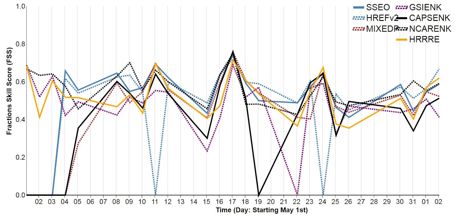
and aggregated across the days for each hour:

give a preliminary metric of each ensembles' performance. The FSS looks at the number of gridboxes covered by a phenomenon (in this case, reflectivity) within a certain radius in the forecast and the observations, therefore eliminating the problem of double penalization incurred when a phenomenon is slightly displaced between the forecasts and the observations. The closer the score is to one, the better it is. Now, there are some data drop-outs in this preliminary data, but it still looks as though the SSEO is performing better than most other ensembles. Aggregated scores across the experiment place the SSEO first, with an FSS of .593. The HREFv2, which is essentially an operationalized SSEO with some differences in the members, was second, with an FSS of .592. Other high-performing ensembles include the NCAR ensemble (.580) and the HRRR ensemble (.559). Again, this data is preliminary, and these numbers will likely change as the cases that didn't run on time in the experiment is rerun.

As for what SFE 2018 will hold, discussions are already underway. Expect to see more of the CLUE, FVGFS, and NEWS-e. A switch-up in how the subjective evaluations are done and revamp of the website is also in the pipeline. Even as the data from SFE 2017 begins to be analyzed, we look forward to SFE 2018 and how we can continue to improve the experiment. Ever onward!

Revisiting the Isochrones

One of the innovations introduced last year was the drawing of isochrones, or lines of equal time. These isochrones indicate the start time of the four-hour period where 95% of the reports at a point were expected to occur - each point has one four-hour period. This year, to aid in the drawing of the isochrones, participants now also draw hourly report coverage areas each hour from 18Z to 03Z. The final product looks something like this forecast from 25 May 2017:

The above image says that the area to the east of the 19Z line will see its most severe weather from 1900 UTC - 2300 UTC, and the areas east of the 23Z line will see the peak severe weather from 2300 UTC - 0300 UTC the following day. Ideally, these lines will be displayed on the 15% threat area (the "slight" risk equivalent) to determine the eastern bound of the final line - currently participants and the NSSL desk lead have this forecast as a background when drawing their isochrones.

Evaluating the Forecast Evolution

Every year in the SFE, a fundamental problem arises when evaluating the long-range full-period forecasts: how to rate the long-range full period forecasts. On the Innovation Desk, participants are given the chance to issue Day 3 forecasts in addition to their day 1 forecast, if time and the potential warrants. Due to the weekly structure of the SFE (which runs M-F), at best two of these forecasts can be evaluated each week - those issued on Monday for Wednesday, and those issued on Tuesday for Thursday. Luckily, with a relatively active period of severe weather CONUS-wide, the three weeks of the experiment so far have yielded evaluations for four out of the potential six days that have Day 3 forecasts. Two of these forecasts give examples of how the long-range forecasts can change as the day of the event draws nearer, and more guidance becomes available: 10 May 2017 and 18 May 2017.

Mind the Gap

Continuing on the last post's theme of choosing the proper forecasting domain when we have multiple areas of convection to contend with, today's discussion will focus on the boldest of forecasting moves:

The gap.

The full period forecasts issued by each desk are a group effort, with input from participants guiding the placement of the lines. Prior to issuing the lines, participants consider observations, coarse-scale operational models such as the GFS and the NAM, and fine-scale operational and experimental models, such as the HRRR, FVGFS, and the members of the CLUE ensemble. Convection-allowing models, with grid spacing of ~3 km, provide very realistic-looking radar signatures that can give confidence in specific areas of threat beyond those of the GFS. For a quick example, see the GFS forecast for 18 May 2017 at 0000 UTC:

The echos from the HRRR suggest that these storms would be supercells, given the strong tracks of  hourly updraft helicity (as indicated by the black contours) and the individual reflectivity echoes. Images such as these can give forecasters more confidence in the location(s) of convection, particularly when compared to the larger-scale QPF precipitation products that current coarse-resolution models can provide. 

So what does this have to do with gapping the forecasts? And what does gapping the forecasts even mean?

Picking Areas during an Active Week

This week is gearing up to be the most active week thus far in the SFE, with every day having the chance of severe weather somewhere in the center of the country. Yesterday, we had three separate areas of potential severe weather to consider:

The first area was concentrated across northern Iowa and far southwestern Wisconsin, the second area stretched from central Nebraska south through western Oklahoma, and the third area was in western South Dakota. Since SFE forecasts cover a subset of the contiguous United States, choosing which areas to forecast for is an important part of the forecast process. In this case, the worst severe convection was anticipated within the eastern two areas, and the forecast domain was chosen to encompass as much of those areas as possible.

CAM Guidance in a Mixed-Mode Case

Yesterday, 11 May 2017, gave the participants in SFE 2017 many things to consider. A potent upper-level low pressure system was finally evolving eastward, after giving the Experiment interesting weather to forecast all week while sitting over the southwest. As the experiment began, ongoing elevated convection was already producing reports over northeastern Oklahoma, and the participants were eyeing the chance for some severe weather locally.

By 2000 UTC (3PM CDT, near the end of the SFE's daily activities), cellular convection was initiating all across northern Oklahoma, northern and western Arkansas, and northeast Texas. Many of these storms quickly began to rotate.

The Denver Hailstorm, 8 May 2017

If you have an interest in severe and unusual weather, you probably already know all about the hailstorm that struck Denver on Monday afternoon, shattering windows and damaging vehicles and roofs across the metro. Indeed, it made for quite the exciting Monday in the Spring Forecasting Experiment.

During the morning forecast discussion, participants noted that good forcing was present over Colorado, along with dewpoints considered sufficient for severe convection by Colorado standards (in the 50's). The moisture was modified Gulf moisture, arriving in CO by way of the Rio Grande thanks to the surface front that was the focus of most of last week's severe convection. Also noted was the unidirectional shear, as can be seen on this 1200 UTC (7:00AM CDT) hodograph from Albuquerque, which was upstream of Denver at 250mb and 500mb.

Verification Determination

Verification is a huge part of the Spring Forecasting Experiment. Each day, we make multiple forecasts on different time scales (this year ranging from daylong outlooks to hourly probabilistic forecasts), and the first activity participants undertake on Tuesday-Friday is an evaluation of the previous day's forecasts. Additionally, in the afternoon, participants evaluate numerical guidance, by comparing model output to observations.

Selecting how to use observations for verifying some of the more nebulous aspects of severe convective weather is one of the challenges of designing the SFE. With some fields, it is easy enough to compare the simulated with the observed - take reflectivity, for example:

Snow Forecasting Experiment??

Strange considerations can crop up in the SFE. In previous years we have forecasted in areas of low radar coverage such as the mountain west, determined which side of the U.S.-Mexico border a storm would form on, and dealt with the severity of convection coming onshore from the Gulf. However, remnants of last weekend's storm threw a highly unusual wrinkle in the forecast....

CLUEing in on Spring Forecasting Experiment 2017

It's nearly the beginning of May (even if it doesn't feel like it in Norman, OK, with a current windchill of 38°F!) and that means that another Spring Forecasting Experiment is about to be underway. This year the Community Leveraged Unified Ensemble (CLUE) is an even more vast than last year, comprised of 81 members from organizations such as NSSL, CAPS, OU, NOAA's Earth Systems Research Laboratory/Global Systems Division (ESRL/GSD), NCAR, and GFDL. These members will provide forecasts of 36 h to 60 h in length, depending on the subsets of the ensemble being considered.

The SFE at the American Meteorological Society's Annual Meeting

During the week before last, over 4500 meteorologists convened in Seattle, Washington for the 97th American Meteorological Society (AMS) annual meeting. As always, I left this meeting with a plethora of new ideas, enthusiasm for the field, and at least a dozen papers added to my to-read pile. However, I also noticed a number of talks which mentioned the Spring Forecasting Experiment, including results from past experiments and hints of what's to come in SFE 2017.

A view of Puget Sound from the Washington State Convention Center, home of the 2017 AMS Annual Meeting

A Late November Outbreak

Greetings from the off-season!

While SFE 2017 (!) is a ways off yet, preparations are already underway for many of the collaborators that provide products to the experiment. Development of the ensembles and guidance tested in the SFEs often occurs across a number of years, as tweaks suggested by prior experiments are implemented alongside new product development.

For example, in SFE 2015 four sets of tornado probabilities were evaluated. While all of the probabilities used 2-5 km updraft helicity (UH) from the NSSL-WRF ensemble, they differed in the environmental criteria used to filter the UH (i.e., if a simulated storm from a member was moving into an unfavorable environment, it was less likely to form a tornado and therefore the ensemble probabilities were lowered). These probabilities showed an overforecasting bias in the seasonally aggregated statistics, and the bias was consequential enough to be noted in subjective participant evaluations. The most typical rating for the probabilities was a 5 or 6 on a scale of 1-10, leaving much room for improvement.

To improve these tornado probabilities, a set of climatological tornado frequencies given a right-moving supercell and a significant tornado parameter (STP) value, as calculated by forecasters at the SPC, were brought to bear on the problem. The application of the climatological frequencies grounded the probabilities in reality. For example, in the prior probabilities if 6/10 ensemble members had a simulated storm passing over the same spot, the forecast probability would be 60%. The updated probabilities consider the magnitude of the STP in the environment the storm is moving into in each member. For example, if all of the storms were moving into an environment with an STP of 2.0, each member is assigned the climatological frequency of a storm to produce a tornado in that situation as the probability of a tornado. Then, the probabilities are averaged across each member. Assuming that 6/10 members now have the storm moving into an environment with STP = 2, the probability would be 60% * the climatological frequency of a tornado given STP = 2. This approach lowers the probabilities, and thus reduces overforecasting.

The new set of probabilities will be tested in SFE 2017. However, these probabilities have been worked on for over a year, and are already available daily on the NSSL-WRF ensemble's website.

While the statistics for all of the tornado probabilities discussed herein were aggregated over the peak of tornado season (i.e., April-June), the end of November 2016 brought tornadoes to the southeastern United States, and with them, the chance to test the new probabilities. We'll focus specifically on 29 November 2016, a day that saw 44 filtered tornado local storm reports (LSRs):

The Storm Prediction Center had a good handle on this scenario, showcasing the potential for severe weather across some of the affected region four days in advance. At 0600 UTC on the day of the event, their "enhanced" area covered much of the hardest-hit areas, with the axis of the outlook a bit skewed from the axis of the LSRs. The outlook and LSRs are shown below.

The 0600 UTC outlook is shown here, because that is when the probabilities computed above become available - our hope is that someday forecasters can look at these probabilities as a "first-guess", encompassing multiple severe storm parameters from the ensemble into one graphic. The SPC's probabilistic tornado forecast from 0600 UTC encompassed all of the tornado reports, but was a bit too far west initially. Ideally, the ensemble tornado forecasts would resemble the SPC's forecast:

When we consider the UH-based probabilities, there's a pocket of high probabilities, between 25-30%, in an area that is close to the highest density of tornado reports. Additionally, all of the reports are not encompassed by the probabilities, and there is an extraneous blob of 5% risk over the DC/Maryland area. The 10% corridor of the probabilities extends further north than the SPC's, but overall, this was a decent forecast, if a bit high in that "bulls-eye" of probabilities. 

Let's compare this to the STP-based probabilities:

These probabilities have a much lower magnitude, but still encompass most of the tornado reports within the 10% contour. The 2% contour is also extended westward into Louisiana, capturing the tornado report that the prior probabilities missed. Overall, this forecast is more like the SPC's outlook, and better reflects what happened on the 29th.

Will we see the same trends into the spring? Aggregated seasonal statistics from spring 2014-2015 seem to suggest yes. However, the opportunity to get participant reflection and evaluation on these probabilities and this methodology awaits - and I, for one, am excited to see what new insights our participants will bring.

SFE 2016 Wrap Up

Well, last week concluded SFE 2016. This season was a particularly interesting one. While we always deal with some marginal cases and mesoscale forcing as the mechanism for severe convection, this year seemed to feature many of those cases. Lots of days throughout the experiment were a bit difficult to forecast conceptually, even the high-end days such as 26 May. While the full period forecasts were easier, breaking down the full period into specific four-hour chunks proved challenging, given that these forecasts contained both a forecast of convective initiation/intensification (if the convection was ongoing) of severe storms, as well as the motion and evolution of those storms (i.e., would supercells form and merge into an MCS? Would morning convection reintensify?). Each of those elements is a forecast challenge separately, but we combined them into one.

In a way, it's ideal that we faced so many of these environments. We've seen in past SFEs that when the CAMs are strongly forced, they often do quite well at pinpointing the location and intensity of severe convection. Where do they have the most difficulty? Under weaker forcing, when remnant outflow boundaries and mesoscale details have a large influence on the day's convection. To have a 65-member CAM ensemble in the CLUE operating during these environments may give us unparalleled insight to what CAM ensemble design characteristics perform best under uncertain circumstances, and can augment the deterministic guidance that is already operational. While we may have come into most days looking at only a small area where CAPE, shear, and a lifting mechanism were present, this set of days will provide us with many case studies of realistic, less-than-ideal circumstances.

As always, a huge thanks goes out to our participants, who hailed from multiple countries and states. We gathered a number of subjective impressions from these participants on various subsets of the CLUE, illustrating forecaster and researcher insights about how these CAMs may best be applied. In the case of the isochrones, this year's comments will help design a better, more user-friendly product and introduction to the concept for next year.

Two great challenges lie ahead: the verification and analysis of the massive amount of data generated and collected during SFE 2016, and the planning of SFE 2017. Such is the cycle of an annual experiment - the work is never done. Onward!

Chopping the FAR

Afternoons in the SFE are composed of three main parts: A Day 2 forecast, evaluations of various aspects of the CAMs, and updates to the morning forecasts. Sometimes, very little new information contributes to these updates, particularly if convection has not initiated by the time of the update. Other days, convective initiation or intensification has occurred, and we have a much better concept of how the convection will evolve. Yesterday was an excellent example of how the afternoon updates can improve upon the morning forecasts, once we get a sense of the evolution.

Data Driven

Well, we have arrived at the fifth and final week of SFE 2016. By this point in the experiment, the facilitators are mostly used to the rhythm of the testbed, knowing what observational data and model guidance we'll go over each day. By the end of the week, participants are generally used to the fast pace of the experiment as well. However, the first day of each week provides some reminders as to how much we're throwing at the participants. I thought that tonight, I'd provide a brief rundown of what we consider when making our full period outlooks each day, which run from 16Z of any given day to 12Z the following day.

CLUE Comparisons

Each day, an evaluation takes place on the total severe desk to compare three subensembles of the CLUE. One subensemble contains 10 ARW members, one contains 10 NMMB members, and one contains 5 ARW and 5 NMMB members. Participants look at two fields to evaluate these subsets of the CLUE: the probability of reflectivity greater than 40 dBZ, and the updraft helicity. This week, all ensembles have been having trouble with grasping the complex convective scenario, as have most of the convection-allowing guidance. However, today's comparison highlighted the challenges of these evaluations: each model had different strengths at varying time periods throughout the forecast, but participants had to provide one summary rating for the entire run.

Model Solutions Galore

This week we've been experiencing broader risk areas in the Spring Forecasting Experiment than previous weeks. The instability has recovered across much of the Great Plains, and the persistent southwesterly flow at upper levels due to a trough in the west has sent steep lapse rates over a wide area. While the trough is still somewhat too far west for the greatest flow to coincide with a broad area of instability, deep-layer shear has been sufficient for severe storms to occur somewhere each day. Determining the exact location is a daily difficulty for our SFE participants.

When we have large areas to consider in conjunction with the huge amount of NWP data we have from the CLUE, deterministic CAMs, and operational large-scale guidance, the number of different scenarios can be overwhelming. Particularly this week, there are multiple solutions for how the day's weather could evolve, according to the NWP. Mesoscale details from prior convection have also played a large role both today and yesterday in making our forecasts, and the variation in the CAM guidance reflects the reliance on those small-scale details. One member's outflow boundary is likely not in the same place as another's, and it's up to participants to determine which solution we think will verify. As an example of the different solutions we saw yesterday, here's a snapshot of five ensemble members whose configuration differs only in the microphysics scheme they're using. Observations are in the lower right hand panel:

Back to the "Basics"

Each day in the Spring Forecasting Experiment, before we consider any numerical weather prediction, participants hand analyze surface and upper air maps. While hand analysis is less common in the digital age, it's an important aspect of our daily routine. Why, you might ask? Well, what do you do when two model runs give you something like this:

Verification (with Low Population)

The target area yesterday was very small, hugging the U.S.-Mexico border from the Big Bend region of Texas northward and westward to New Mexico. This area is sparsely populated, which becomes an issue when trying to verify forecasts of severe weather. The United States is far from the only country to have this problem - one participant gave a talk this week that mentioned how the area with the most severe weather in South America is also sparsely populated. When we're forecasting for an underpopulated area in the experiment we have to examine metrics other than Local Storm Reports (LSRs), particularly because the verification of yesterday's forecasts is the first activity each morning.